Particle Swarm Optimization
- Gianluca Turcatel

- Jan 2, 2022
- 5 min read

Introduction
Particle swarm optimization (PSO) is a very well establish computational method that optimizes a problem by iteratively improving a candidate solution with regard to an objective function. PSO is a meta-heuristic optimization algorithm, which means it is problem-independent techniques. Therefore, it won't take advantage of any specificity of the problem and can be used as black box.
PSO is a stochastic, population-based algorithms and utilizes a population of candidate solutions, named particles, that move around in the search-space seeking for the global optimum.
The movement of each particle is dictated by 3 components (Figure 1):

Figure 1. Particle's movement in PSO algorithm - Part 1
The particle's movement is dictated by its previous moves (purple arrow), its own best known position (red arrow), and the best known position among all particles in the swarm(green). The sum of these there forces dictates where the particle will land in the next iteration (Figure 2):
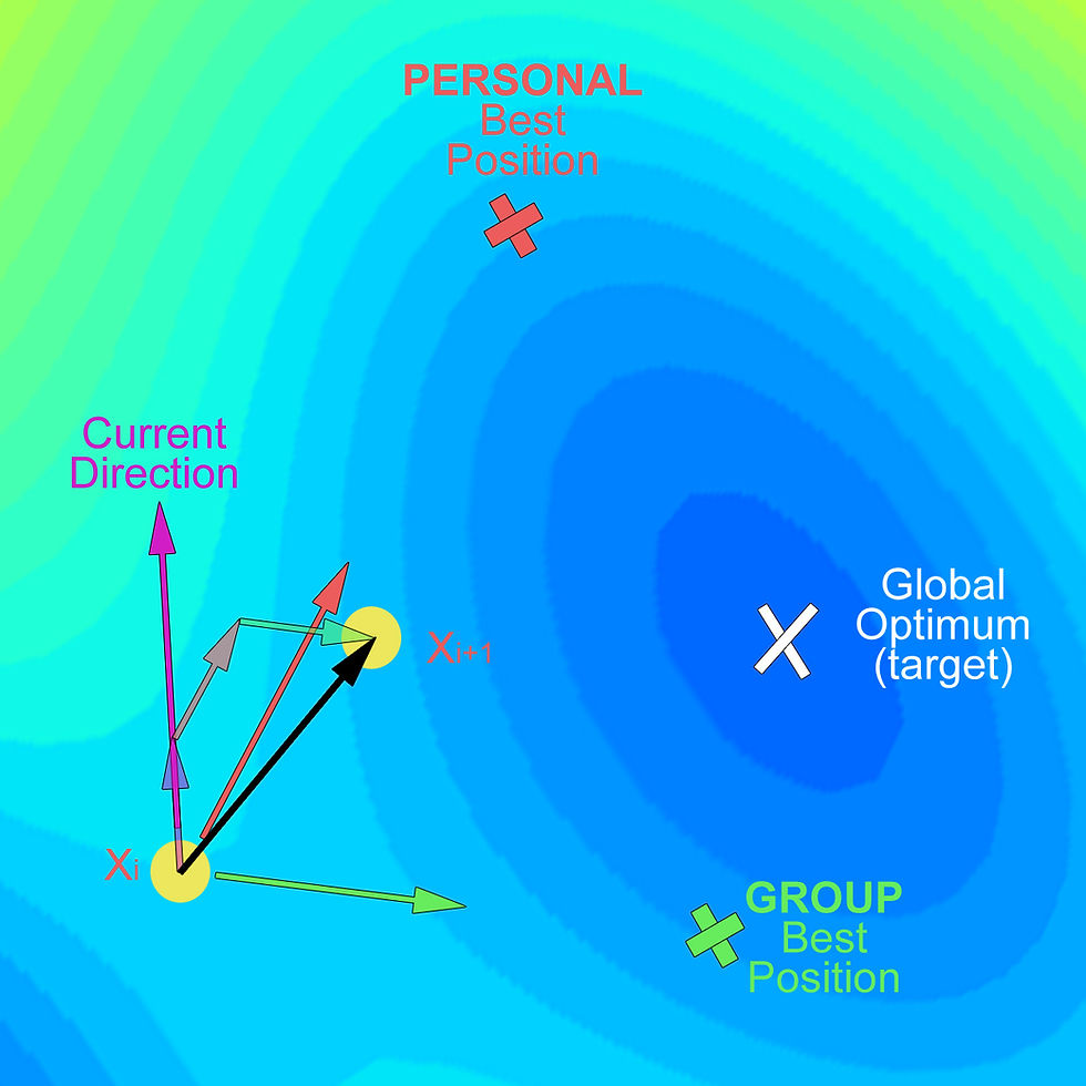
Figure 2. Particle's movement in PSO algorithm - Part 2
In the next iteration, let's assume the group best position improved a little:
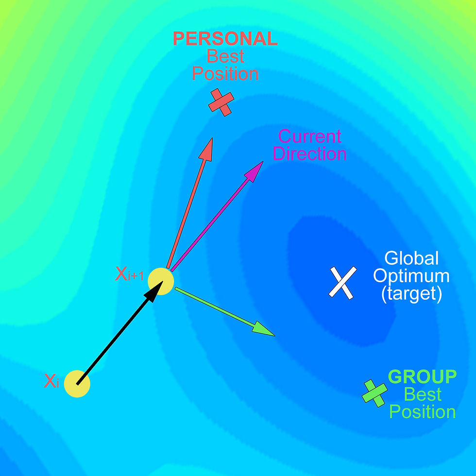
Figure 3. Particle's movement in PSO algorithm - Part 3
In figure 3, note that current direction is given by the previous move. In then next step, the particle will land at Xi+2, again, according to the sum of the 3 vectors (Figure 4):

Figure 4. Particle's movement in PSO algorithm - Part 4
In Figure 1-4 I showed the moves of one single particle. Imagine this happening for several particles: after a certain amount of iterations, the swarm of particles will concentrate on the global minimum. Why does the algorithm find the optimum position? Because the particles keep track of the best personal and global positions and search around them, the chance of finding a better position is high, eventually pulling the particles to hit the target.
PSO - The Math:
Assuming P particles, the position of the particle i at the time t is denoted by a vector of length d:

At every iteration each particle's position is updated according to the equation:

The position of the particle at the next iteration is equal to its current position plus the velocity vector which is given by:

Vi is the current direction of the particle, Pi is the particle's best personal location, and Gi is the group's best location. r1 and r2 are random numbers between 0 and 1: the fact that r1 and r2 are sampled at each iteration makes the PSO a stochastic algorithm. w (inertia weight), c1 and c2 are hyperparameters. w tunes exploration and exploration. c1 and c2 affect the impact of the individual and global component on particle's velocity.
Each term in (3) have its own name:

The inertia component carries forwards the direction of the particle's move from the previous iteration; the individual (or cognitive) term compares the particle current position with its own best position; the social component calculates the distance between the current particle location and the best position of the whole swarm.
Implementation
The figure below depicts the landscape the particles will explore. The global minimum is located around the center of the figure (white cross).

Figure 5. Objective function landscape
Below you will find the python code of the PSO algorithm. The Jupyter Notebook can be found HERE.
def particle_swarm(n_iterations, w, c1, c2,
                   n_particles, x, y, loss_function):

    # Calculate Z
    X, Y = np.meshgrid(x, y)
    Z = loss_function(X, Y)

    # Find the location of the global minimum
    x_min = X.ravel()[np.argmin(Z)]
    y_min = Y.ravel()[np.argmin(Z)]
    min_tuples = (x_min, y_min)

    # Empty dictionary to store particle information
    particle_positions = {}

    # Get the range of x and y
    x_lim_min, x_lim_max = np.min(x), np.max(x)
    y_lim_min, y_lim_max = np.min(y), np.max(y)

    # Random initialization of particles' starting position
    particles_x =np.random.rand(n_particles) * (x_lim_max - x_lim_min) - \
    x_lim_max

    particles_y =np.random.rand(n_particles) * (y_lim_max - y_lim_min) - \
    y_lim_max

    start_position_particles =np.concatenate([particles_x.reshape(-1,1), \
    particles_y.reshape(-1,1)], axis = 1)

    # Initial random velocity of the particles
    start_velocity = np.random.normal(size = (n_particles, 2)) * 0.5

    # Initially, the best individual position is the starting position
    best_personal_position = start_position_particles

    # Calculate best group position
    loss = loss_function(start_position_particles[:,0], \
    start_position_particles[:,1])

    best_group_location = start_position_particles[np.argmin(loss),:]

    # Storing start position, best_personal_position, initial velocity,
    # best_group_location
    particle_positions[0] = [start_position_particles,
                             best_personal_position,
                             start_velocity,
                             best_group_location]

    # Main loop
    for iteration in range(n_iterations):

        # Give random value to  r1 and r2
        r1, r2 = np.random.rand(2)

        # Extract previous iteration values
        current_position = particle_positions[iteration][0]
        current_velocity = particle_positions[iteration][2]
        current_best_personal_position = particle_positions[iteration][1]
        current_best_group_position = particle_positions[iteration][3]

        # Calculate velocity at next iteration
        V_next = w * current_velocity + \
        c1*r1*(current_best_personal_position - current_position) + \
        c2*r2*(current_best_group_position - current_position)

        # Calculate position at next iteration
        x_next = current_position + V_next

        # Calculate current and next position's loss
        previous_loss = loss_function(current_position[:,0], \
        current_position[:,1])
        next_loss = loss_function(x_next[:,0], x_next[:,1])
        losses = np.concatenate([previous_loss,next_loss])

        # Update best personal position
        update_personal_best_indexes = \
        np.argmin(losses.reshape(2,n_particles), axis = 0)

        previous_next_position_concat = \
        np.concatenate([np.expand_dims(current_position, axis = 1),
                        np.expand_dims(x_next, axis = 1)], axis =1)

        next_best_personal_position = previous_next_position_concat[ \
        np.arange(n_particles),update_personal_best_indexes,:]

        # Calculate current and next best group position
        current_best_group_location_loss =
        loss_function(current_best_group_position[0],
        current_best_group_position[1])

        next_best_group_location = x_next[np.argmin(next_loss),:]
        next_best_group_location_loss = np.min(next_loss)

        # Update best group position
        if current_best_group_location_loss<next_best_group_location_loss:
            next_best_group_location = current_best_group_position

        # Storing new values in the dictionary
        particle_positions[iteration + 1] = [x_next,
                                             next_best_personal_position,
                                             V_next,
                                             next_best_group_location]

    # Plot location and velocity of particles at 6 iterations
    delta = round((n_iterations-1) / 5 )
    indexes_to_plot = list(range(0, n_iterations, delta ))
    indexes_to_plot.append(n_iterations)
    cols = 2
    rows = 3

    # Create the figure
    plt.figure(figsize = (8*cols,6*rows))

    # For loop for the subplots
    for num, ind in enumerate(indexes_to_plot):
        current_position = particle_positions[ind][0]
        current_position_velocity = particle_positions[ind][2]
        plt.subplot(rows,cols , num+1)
        plt.title(f"Iteration: {ind}")
        # Plot the contours
        plt.contourf(X, Y, Z, 50, cmap='jet')
        # Plot the particles' location
        plt.scatter(current_position[:,0], current_position[:,1], color =
        'red')
        # Plot the particles' velocity
        plt.quiver(current_position[:,0].ravel(),
                   current_position[:,1].ravel(),
                   current_position_velocity[:,0].ravel(),
                   current_position_velocity[:,1].ravel(),
                   color='blue', width=0.005, angles='xy',
                   scale_units='xy', scale=1)
        # Display the location of the minimum
        plt.plot(x_min, y_min, marker = 'x', color = 'white', \
        markersize = 10, label = 'minumum')
        plt.xlim([x_lim_min, x_lim_max])
        plt.ylim([y_lim_min, y_lim_max])
        plt.colorbar()

    plt.tight_layout()
    plt.show()

    # Return the dictionary with the particles' history
    return particle_positions
Let's test the PSO algorithm with 30 particles, 30 iterations, w = 0.5, c1=c2=0.1:

Figure 6. PSO algorithm result
After 30 iteration, the particles successfully concentrated tightly around the optimum's location as we wanted. The animation below displays the movement of the particles at each iteration (* indicates the group's best location:
Figure 7. PSO algorithm result - animation
Concluding remarks
In this article the inertia weight w was kept constant; however, it is not uncommon to decrease its value at each iteration (for instance from an initial value of 0.9 to a final value of 0.4). Lowering w will force the particles to explore less and focus more on individual and collective best locations.
PSO does not require calculating the derivative of the objective function in contrast to gradient descent, which makes it the preferable optimization algorithm when the derivative of the objective function is hard to derive. Furthermore, because it has a relative low number of hyperparameters, PSO is easy to tune and implement, and can solve a wide range of problems.


Comentarios